Choosing a density estimator

npe() approximates the posterior with a conditional density estimator: a model of p(theta | x) trained on simulated (theta, x) pairs. The density_estimator argument picks which one, and the choice matters most when the posterior is non-Gaussian. This vignette describes the four options and when each is the right choice.

The four estimators

• "linear_gaussian" — a closed-form conditional Gaussian fit by linear regression. No neural network and no torch. It is exact when the true posterior is Gaussian in the parameters, which makes it both a fast baseline and a sanity check for the neural estimators.
• "mdn" — a mixture density network: a small neural network that maps x to the weights, means, and covariances of a Gaussian mixture. Mixtures can represent multimodal and skewed posteriors, and training is quick.
• "maf" (the default) — a masked autoregressive flow (Papamakarios et al., 2017): builds the posterior density from a sequence of invertible transformations of a Gaussian. More flexible than a mixture when the parameters have strong nonlinear dependence. This is also the default in Python sbi.
• "nsf" — a neural spline flow (Durkan et al., 2019): a flow whose transformations are monotonic splines. The most flexible of the three, at somewhat higher training cost.

All three neural estimators need the torch back end (install.packages("torch"); torch::install_torch()) and share one training loop, so the training arguments to npe() — max_epochs, patience, n_restarts, and so on — mean the same thing whichever you pick.

A posterior no Gaussian can fit

The two-moons benchmark task has a bimodal, crescent-shaped posterior. It is built into the package:

library(neuralsbi)
#> 
#> Attaching package: 'neuralsbi'
#> The following object is masked from 'package:base':
#> 
#>     sample

task <- task_two_moons()
task
#> <nsbi_task> two_moons: 2 parameters -> 2 data dims

x_obs <- c(0, 0)

The linear-Gaussian estimator cannot represent two modes; it returns a single wide Gaussian that averages across both:

fit_lg <- npe(task$prior, task$simulator, n_simulations = 2000,
              density_estimator = "linear_gaussian", seed = 1)
draws_lg <- sample(posterior(fit_lg, x_obs = x_obs), 3000)
pairplot(draws_lg)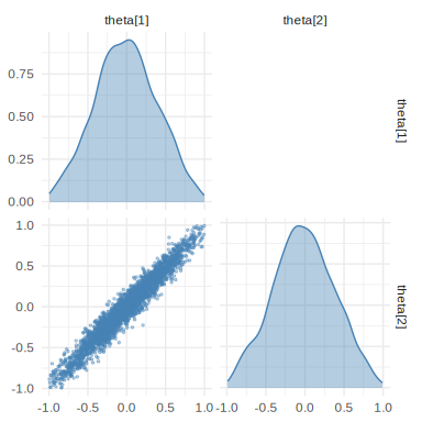

plot of chunk unnamed-chunk-3

The MDN, with its mixture components, recovers both moons:

fit_mdn <- npe(task$prior, task$simulator, n_simulations = 2000,
               density_estimator = "mdn", n_components = 10,
               max_epochs = 200, seed = 1)
draws_mdn <- sample(posterior(fit_mdn, x_obs = x_obs), 3000)
pairplot(draws_mdn)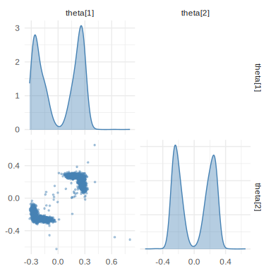

plot of chunk unnamed-chunk-4

And a spline flow captures the sharp crescent edges most cleanly:

fit_nsf <- npe(task$prior, task$simulator, n_simulations = 2000,
               density_estimator = "nsf", max_epochs = 150, seed = 1)
draws_nsf <- sample(posterior(fit_nsf, x_obs = x_obs), 3000)
pairplot(draws_nsf)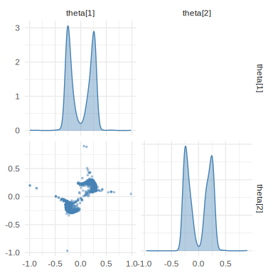

plot of chunk unnamed-chunk-5

Comparing estimators quantitatively

A classifier two-sample test (c2st()) measures how distinguishable two sets of samples are: 0.5 means the classifier cannot tell them apart, 1.0 means it always can. The MDN and the flow agree closely here — both recover the two moons, so a classifier is near chance:

c2st(draws_mdn, draws_nsf, seed = 1)$accuracy   # near 0.5: MDN and NSF agree
#> [1] 0.513

The linear-Gaussian fit is visibly wrong — one blob instead of two crescents — yet c2st() does not flag it:

c2st(draws_lg, draws_nsf, seed = 1)$accuracy    # also near 0.5 (see below)
#> [1] 0.5025

That number is a trap worth understanding. c2st() trains a linear classifier, so it separates samples by their mean and covariance alone. The two moons are symmetric about the origin — the same centre and roughly the same spread as the Gaussian blob — so no straight decision boundary can tell the two sets apart, even though one is bimodal and the other is not. The pairplots above show exactly the difference the score misses. The lesson: a two-sample score is only as sharp as its classifier, and a linear one is blind to multimodality. For that, trust the picture, or a calibration check (vignette("diagnostics")).

When two posteriors differ in their mean or covariance — as an estimated and an exact posterior do for task_gaussian_linear() — the linear classifier detects the gap well, and c2st() is the right tool. That is how the package’s own accuracy tests score estimators against analytic references.

Adjusting flexibility

Each estimator has a few settings, passed through npe(), that control how flexible it is:

Estimator	Arguments	Default
"mdn"	n_components, hidden	5 components, two hidden layers of 50 units
"maf", "nsf"	n_transforms, hidden	5 transforms
"linear_gaussian"	none	—

A more flexible model helps only if there are enough simulations to train it; with a few thousand simulations the defaults are usually right. If the estimated posterior looks too smooth or too wide, adding simulations usually helps more than enlarging the network.

Practical guidance

• The default "maf" matches Python sbi and handles strong nonlinear dependence between parameters. "mdn" trains a little faster and can represent multiple modes.
• If the posterior has sharp features that the MAF or MDN smooth over, switch to "nsf".
• Use "linear_gaussian" when torch is unavailable, when you want a near-instant baseline, or when the model really is linear-Gaussian — then it is exact.
• Whatever you choose, check it. vignette("diagnostics") shows how to verify a fitted posterior with calibration and predictive checks.