neuralsbi and pomp: two routes to an SIR posterior

pomp is the established R toolkit for partially observed Markov process models — the stochastic dynamical systems common in epidemiology and ecology. It fits them by particle filtering: a sequential Monte Carlo scheme that only ever simulates the latent state process, so you never write down its transition density. That makes pomp simulation-based in the same spirit as neuralsbi. The two packages differ in what they do next, and this vignette puts them on the same problem to see whether their posteriors agree.

The problem is a stochastic SIR epidemic. A population of size N splits into Susceptible, Infected, and Recovered; the contact rate $\beta$ drives new infections and the recovery rate $\gamma$ drives recoveries. We infer $(\beta, \gamma)$ from a single noisy incidence curve. The dynamics are genuinely stochastic — infections and recoveries are random events, not a smooth ODE — so there is no tractable likelihood for the observed curve.

(A note on notation: SBI writes the observed data $\mathbf{x}$, the role regression gives to $y$. Here $\mathbf{x}$ is the reported-case time series.)

The model, written twice

Both packages need the same generative model. pomp wants it as C snippets; neuralsbi wants a vectorized R function. The dynamics are identical: an Euler step with binomial transitions, and reported cases drawn as a binomial thinning of the true weekly incidence.

library(pomp)

sir_step <- Csnippet("
  double dN_SI = rbinom(S, 1 - exp(-Beta * I / N * dt));  // new infections
  double dN_IR = rbinom(I, 1 - exp(-gamma * dt));         // new recoveries
  S -= dN_SI;
  I += dN_SI - dN_IR;
  R += dN_IR;
  H += dN_SI;                                             // accumulate incidence
")

sir_rinit <- Csnippet("S = N - I0; I = I0; R = 0; H = 0;")

# pomp needs BOTH the measurement simulator (rmeasure) and its DENSITY
# (dmeasure): the particle filter has to evaluate p(reports | H).
rmeas <- Csnippet("reports = rbinom(H, rho);")
dmeas <- Csnippet("lik = dbinom(reports, H, rho, give_log);")

Fixed settings and the true rates that generate our observation:

N <- 1000; I0 <- 10; rho <- 0.5; Tobs <- 20
theta_true <- c(Beta = 2, gamma = 1)      # basic reproduction number R0 = 2

We assemble the pomp object and simulate one outbreak. That simulated curve is the data both methods will condition on.

sir <- pomp(
  data       = data.frame(time = 1:Tobs, reports = NA),
  times      = "time", t0 = 0,
  rprocess   = euler(sir_step, delta.t = 1/10),
  rinit      = sir_rinit,
  rmeasure   = rmeas, dmeasure = dmeas,
  accumvars  = "H",
  statenames = c("S", "I", "R", "H"),
  paramnames = c("Beta", "gamma", "rho", "N", "I0")
)

pars  <- c(theta_true, rho = rho, N = N, I0 = I0)
x_obs <- as.numeric(obs(simulate(sir, params = pars, seed = 12345)))
sir@data <- matrix(x_obs, nrow = 1, dimnames = list("reports", NULL))

plot(1:Tobs, x_obs, type = "b", pch = 16,
     xlab = "week", ylab = "reported cases", main = "Observed outbreak")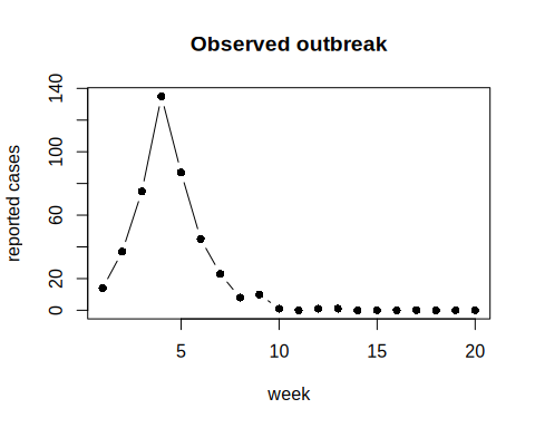

plot of chunk unnamed-chunk-4

Route 1 — pomp: particle-filter MCMC

The particle filter estimates the likelihood at any parameter value by propagating a swarm of simulated state trajectories and weighting them by dmeasure.

logLik(pfilter(sir, params = pars, Np = 1000))   # unbiased log-likelihood estimate
#> [1] -39.34408

For a Bayesian posterior, pmcmc embeds that filter inside a Metropolis-Hastings sampler. We put uniform priors on the two rates — the same priors neuralsbi will use — and run a short adaptive chain.

sir_bayes <- pomp(sir,
  dprior = Csnippet("
    lik = dunif(Beta, 0.5, 5, 1) + dunif(gamma, 0.2, 3, 1);
    lik = give_log ? lik : exp(lik);"),
  paramnames = c("Beta", "gamma"))

set.seed(1)
chain <- pmcmc(sir_bayes, Nmcmc = 2000, Np = 500, params = pars,
               proposal = mvn_rw_adaptive(rw.sd = c(Beta = 0.1, gamma = 0.05),
                                          scale.start = 100, shape.start = 200))

post_pomp <- as.data.frame(traces(chain))[501:2000, c("Beta", "gamma")]  # drop burn-in
round(colMeans(post_pomp), 3)
#>  Beta gamma 
#> 2.075 0.852
round(apply(post_pomp, 2, sd), 3)
#>  Beta gamma 
#> 0.221 0.168

The chain concentrates around the true rates. This posterior is specific to this one outbreak: a different curve means running the sampler again.

Route 2 — neuralsbi: neural posterior estimation

neuralsbi never evaluates a measurement density. It only needs to draw from the model, so we write the same dynamics as a vectorized simulator: an $n \times 2$ matrix of parameters in, an $n \times 20$ matrix of reported curves out.

library(neuralsbi)
#> 
#> Attaching package: 'neuralsbi'
#> The following object is masked from 'package:base':
#> 
#>     sample

sir_simulator <- function(theta) {
  n <- nrow(theta); Beta <- theta[, 1]; gamma <- theta[, 2]
  S <- rep(N - I0, n); I <- rep(I0, n); R <- rep(0, n)
  out <- matrix(0, n, Tobs)
  for (tt in seq_len(Tobs)) {          # one column per week
    H <- rep(0, n)
    for (s in seq_len(10)) {           # ten Euler substeps, dt = 1/10
      dN_SI <- rbinom(n, S, 1 - exp(-Beta * I / N * 0.1))
      dN_IR <- rbinom(n, I, 1 - exp(-gamma * 0.1))
      S <- S - dN_SI; I <- I + dN_SI - dN_IR; R <- R + dN_IR; H <- H + dN_SI
    }
    out[, tt] <- rbinom(n, H, rho)     # binomial reporting
  }
  out
}

Neural Posterior Estimation (NPE) trains a conditional density estimator $q_\phi(\boldsymbol{\theta} \mid \mathbf{x})$ on simulated $(\boldsymbol{\theta}, \mathbf{x})$ pairs, then conditions it on the observed curve. Training is amortized: one fit works for any incidence curve, not just this one. A mixture density network suits this smooth, unimodal posterior.

prior <- prior_uniform(low = c(0.5, 0.2), high = c(5, 3))   # same as pomp's dprior

# 8000 simulations to train a 2-parameter posterior. If it comes out too wide, add simulations before enlarging the network.
fit <- npe(prior, sir_simulator, n_simulations = 8000,
           density_estimator = "mdn", max_epochs = 400,
           n_restarts = 2, seed = 1)

post_npe <- posterior(fit, x_obs = x_obs)
draws_npe <- sample(post_npe, 4000)
round(colMeans(draws_npe), 3)
#> [1] 2.097 0.894
round(apply(draws_npe, 2, sd), 3)
#> [1] 0.347 0.239

Do the posteriors agree?

Overlay the two posterior clouds and score them with a classifier two-sample test (C2ST): an accuracy near 0.5 means a classifier cannot tell the two sets of draws apart.

# thin the NPE draws to pomp's count so neither cloud simply outnumbers the other
npe_thin <- draws_npe[sample(nrow(draws_npe), nrow(post_pomp)), ]
plot(npe_thin[, 1], npe_thin[, 2], pch = 16, cex = 0.5,
     col = adjustcolor("steelblue", 0.35),
     xlab = expression(beta), ylab = expression(gamma),
     xlim = c(1, 3.5), ylim = c(0.3, 1.6))
points(post_pomp$Beta, post_pomp$gamma, pch = 16, cex = 0.5,
       col = adjustcolor("firebrick", 0.4))
points(2, 1, pch = 3, cex = 2, lwd = 2)
legend("topright", c("pomp (pMCMC)", "neuralsbi (NPE)", "truth"),
       col = c("firebrick", "steelblue", "black"), pch = c(16, 16, 3), bty = "n")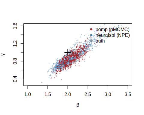

plot of chunk unnamed-chunk-9

c2st(as.matrix(draws_npe), as.matrix(post_pomp), seed = 1)$accuracy
#> [1] 0.7272727

The two posteriors sit on top of each other: same location, same $\beta$–$\gamma$ ridge (the two rates trade off because the data mostly pin down their ratio $R_0$). The C2ST lands well above 0.5, and the plot shows why — the neuralsbi cloud is a little broader. That is the expected signature of the trade-off. pomp’s particle filter exploits the known binomial measurement density to extract the sharpest posterior this dataset supports; NPE is handed only simulations and, at an 8000-simulation budget, stays slightly more cautious. More simulations tighten it toward pomp.

Is that extra width honest or a bug? Simulation-based calibration answers it without a reference posterior: draw $\boldsymbol{\theta}$ from the prior, simulate, and rank the truth among the posterior draws. Calibrated posteriors give uniform ranks.

sbc_res <- sbc(fit, sir_simulator, n_sbc = 150, n_posterior_samples = 300,
               seed = 2)
sbc_res                    # large p-values = calibrated
#> <nsbi_sbc> 150 trials, 300 posterior samples each
#>   per-parameter uniformity p-values (large = calibrated):
#>     0.312  0.181
plot_sbc(sbc_res, param = 1)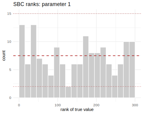

plot of chunk unnamed-chunk-10

The ranks are flat and the p-values large: NPE’s wider intervals are calibrated, not broken. neuralsbi and pomp give the same answer here, and NPE simply reports a touch more uncertainty for the simulations it was given.

Similarities and differences

	pomp (pMCMC)	neuralsbi (NPE)
Latent state process	simulated only	simulated only
Measurement model	needs the density (dmeasure)	needs only to simulate
Inference	particle filter + MCMC	train a neural density estimator
Reusable across datasets	no — refit per observation	yes — amortized
Cost structure	cheap setup, rerun per dataset	expensive training, then instant
Exactness	exact in the MCMC limit	approximate; must be calibration-checked

Reach for pomp when you can write the measurement density and have one or a few datasets to fit — it will give the sharpest, best-understood posterior. Reach for neuralsbi when the measurement model itself is a black box, or when you need to condition on many datasets and amortization pays for the training up front. On this problem they agree, which is the reassuring outcome: two different simulation-based machines, pointed at the same stochastic model, recover the same rates.

For the neuralsbi workflow in more depth, see vignette("neuralsbi") and vignette("diagnostics"); for pomp, the package tutorials.