Checking the posterior

An NPE posterior is an approximation, and a poor approximation gives no warning: it still produces samples, means, and credible intervals — they are just wrong. Checking the fit is part of the workflow, not an optional extra. This vignette works through the package’s diagnostics in the order you would use them in practice.

Throughout we use the linear-Gaussian benchmark task, because it has an analytic posterior we can compare against at the end.

library(neuralsbi)

task <- task_gaussian_linear()
task
#> <nsbi_task> gaussian_linear: 10 parameters -> 10 data dims (analytic reference available)

fit <- npe(task$prior, task$simulator, n_simulations = 3000,
           density_estimator = "linear_gaussian", seed = 1)

Simulation-based calibration

Simulation-based calibration (SBC) checks the posterior on average over the prior, with no reference posterior needed. The idea: draw theta from the prior, simulate x, and rank the true theta among posterior draws given x. If the posterior is calibrated, those ranks are uniform.

res <- sbc(fit, task$simulator, n_sbc = 100, n_posterior_samples = 200,
           seed = 2)
res
#> <nsbi_sbc> 100 trials, 200 posterior samples each
#>   per-parameter uniformity p-values (large = calibrated):
#>     0.444  0.470  0.684  0.326  0.970  0.083  0.684  0.025  0.444  0.735

plot_sbc(res, param = 1)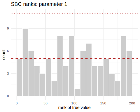

plot of chunk unnamed-chunk-3

Read the rank histogram like this:

• Flat — calibrated.
• U-shaped — the posterior is too narrow (overconfident). The most common failure; usually fixed with more simulations or longer training.
• Hump-shaped — too wide (underconfident).
• Sloped — systematically biased in one direction.

Expected coverage

The same SBC ranks yield a coverage curve: how often does the p% credible interval actually contain the truth?

expected_coverage(res)
#>    nominal param1 param2 param3 param4 param5 param6 param7 param8 param9
#> 1     0.05   0.04   0.04   0.05   0.06   0.05   0.05   0.02   0.02   0.03
#> 2     0.10   0.09   0.09   0.10   0.14   0.10   0.11   0.09   0.09   0.07
#> 3     0.15   0.14   0.12   0.17   0.21   0.14   0.14   0.13   0.13   0.14
#> 4     0.20   0.18   0.19   0.23   0.28   0.20   0.19   0.22   0.18   0.19
#> 5     0.25   0.22   0.28   0.28   0.34   0.22   0.23   0.28   0.27   0.23
#> 6     0.30   0.32   0.34   0.34   0.39   0.26   0.26   0.34   0.29   0.26
#> 7     0.35   0.35   0.37   0.37   0.42   0.27   0.36   0.40   0.34   0.29
#> 8     0.40   0.39   0.39   0.43   0.46   0.33   0.42   0.42   0.36   0.35
#> 9     0.45   0.43   0.45   0.51   0.50   0.38   0.46   0.49   0.43   0.43
#> 10    0.50   0.48   0.53   0.53   0.52   0.46   0.51   0.55   0.53   0.49
#> 11    0.55   0.52   0.58   0.55   0.56   0.53   0.56   0.60   0.57   0.55
#> 12    0.60   0.56   0.60   0.63   0.64   0.59   0.59   0.63   0.59   0.60
#> 13    0.65   0.59   0.65   0.68   0.69   0.69   0.66   0.66   0.64   0.69
#> 14    0.70   0.64   0.71   0.72   0.73   0.73   0.76   0.72   0.69   0.73
#> 15    0.75   0.68   0.76   0.77   0.74   0.77   0.78   0.77   0.71   0.73
#> 16    0.80   0.72   0.78   0.81   0.80   0.83   0.82   0.82   0.76   0.80
#> 17    0.85   0.78   0.84   0.87   0.84   0.88   0.87   0.89   0.82   0.85
#> 18    0.90   0.89   0.94   0.93   0.90   0.90   0.91   0.93   0.84   0.91
#> 19    0.95   0.93   0.94   0.97   0.96   0.93   0.96   0.95   0.90   0.96
#>    param10
#> 1     0.01
#> 2     0.09
#> 3     0.13
#> 4     0.20
#> 5     0.27
#> 6     0.37
#> 7     0.41
#> 8     0.47
#> 9     0.50
#> 10    0.55
#> 11    0.59
#> 12    0.63
#> 13    0.68
#> 14    0.74
#> 15    0.80
#> 16    0.85
#> 17    0.87
#> 18    0.93
#> 19    0.96
plot_coverage(res)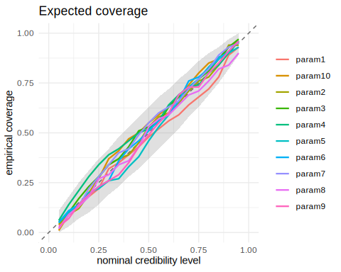

plot of chunk unnamed-chunk-4

A calibrated posterior hugs the diagonal. Points below the diagonal mean intervals are too narrow — a 90% interval that covers the truth only 70% of the time.

TARP: a sharper coverage test

SBC checks each parameter’s marginal. TARP (Lemos et al., 2023) tests coverage of the joint posterior using random reference points, and can detect miscalibration that per-parameter ranks miss.

tr <- tarp(fit, task$simulator, n_tarp = 100, n_posterior_samples = 200,
           seed = 3)
tr
#> <nsbi_tarp> 100 trials, 200 posterior samples each
#>   max |ECP - nominal|: 0.130 (0 = perfectly calibrated)
#>   plot with plot_tarp()
plot_tarp(tr)   # ECP curve on the diagonal = calibrated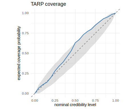

plot of chunk unnamed-chunk-5

Posterior predictive checks

Calibration is an average over many simulated datasets; a predictive check asks about the observation you actually have. Push posterior draws back through the simulator and see whether the observed data look typical of the simulations they produce.

theta_true <- sample_prior(task$prior, 1)
x_obs <- task$simulator(theta_true)

post <- posterior(fit, x_obs = x_obs)
pred <- posterior_predictive(post, task$simulator, n = 500)
plot_posterior_predictive(pred, x_obs)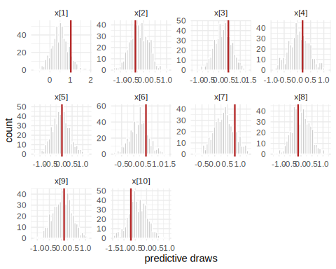

plot of chunk unnamed-chunk-6

If the observation sits in the tails of the predictive distribution, either the posterior fit is poor for this x or the simulator cannot reproduce the data at all — a model-misspecification signal that no calibration check provides.

Comparing against a reference posterior

When a reference posterior exists — analytic, MCMC, or a long-run fit you trust — a classifier two-sample test gives a single accuracy score. A classifier that cannot distinguish estimated from reference draws (accuracy near 0.5) means the posteriors match.

draws     <- sample(post, 5000)
reference <- task$reference_posterior(x_obs, n = 5000)

c2st(draws, reference)$accuracy   # ~0.5: indistinguishable from the exact posterior
#> [1] 0.5519

As a rule of thumb, accuracies below about 0.55–0.6 indicate a close match; values near 1.0 mean the estimated posterior is badly off.

A suggested routine

1. After every fit, run sbc() and look at plot_sbc() and plot_coverage(). This is cheap relative to training and catches overconfidence early.
2. Before using a posterior for real conclusions, run a posterior predictive check for the actual observation.
3. When you change estimator or training settings, compare old and new draws with c2st() to see whether the change moved the posterior at all.

The case study in vignette("sir-epidemic") applies this routine end to end on an applied problem.